Editorial for APIO '10 P2 - Patrol
Submitting an official solution before solving the problem yourself is a bannable offence.
The road network forms a tree . A tree with
nodes has
edges. In
, the length of a tour that visits all edges is
, because each edge is visited twice. Recall that adding edges into a tree creates cycles.
Simpler case
We consider a simpler case when . Suppose that we add edge
to
. The resulting graph
contains exactly one cycle
. The cheapest tour visiting all edges uses each edge in
once and all other edges twice. Denote
as path
. The new length of the required tour is
where is the length of
. Thus, for
, we need to find the maximum path length for paths in
. This value is called the diameter of
.
There are many ways to find the diameter. We shall use dynamic programming, which can be turned into a solution for the general case.
First, we root the tree at some node ; the parent-child relation between adjacent nodes can be defined naturally. For each node
, let
denote the length of the longest path from
to some of its descendants. We can compute
for each
, in
time, using a simple dynamic programming.
Consider the longest path , let node
be the node on
closest to the root
. By definition,
is unique. Given
, the length of
must be either
, if
has one child, or
when has more than one child. The value above is important to the case where
as well, so let's define it as
. Formally,
is the maximum length of paths containing
such that
is the closest node to root
.
Thus by enumerating all nodes, one can find the length of the longest path; thus, one can compute the answer to the case where .
When 
Let's call both edges and
. Let path
be a unique path that joins two endpoints of
, also let's call a unique cycle induced by adding each edge
(separately) as
. Note that
is a union of
and
.
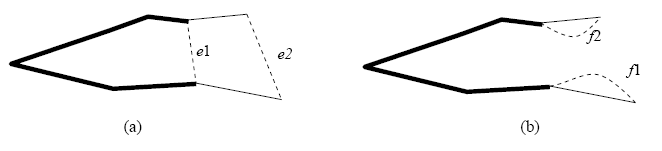
Figure 1: (a) Edges and
are shown as dashed lines. Paths
and
intersect. The intersection is shown as a thick line. In the tour, these edges must still be traversed over twice. (b) The new edges
and
are shown as dashed lines. Note that the number of times each edge on the tree is traversed on is the same as before.
When and
are disjoint, the length of the desired tour that traverses all edges is
where is the length of
.
It gets more complicated when 's intersect. However, since one must traverse on each
exactly once, it is not hard to prove the following claim.
Claim: If and
intersect, there is another pair of edges
and
such that the paths joining each edge's endpoints are disjoint, and the length of the tour traverses all edges in
is the same as in
.
The proof is left out, but Figure 1 illustrates the idea of the proof.
From the claim, to find how to add two edges to minimize the tour, we need to only consider finding a pair of disjoint paths whose sum of lengths is maximum. This, again, can be solved using dynamic programming in time.
Besides , we need other variables. Let
be the subtree rooted at
. We define:
is the maximum length of paths inside
.
is the maximum sum of lengths of any pairs of edge-disjoint paths
and
in
.
Figure 2 shows examples of paths considered in and
.
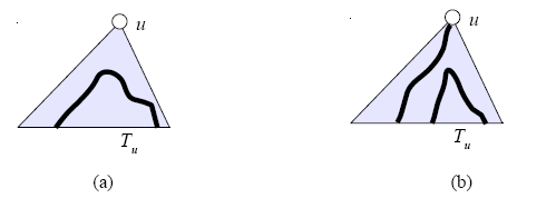
Figure 2: (a) Paths considered in . (b) A pair of paths considered in
.
Let denote the number of children of
on the rooted tree
. It takes
time to compute
from information from its children by taking the maximum of
for all children
of
and
.
To compute , a straightforward implementation takes
time. A careful implementation only takes
time. (See discussion in the next section.)
With 's and
's of all child nodes of
at hand, one can find
the maximum sum of lengths of pairs of paths
and
such that
and
are disjoint,
- Among all nodes in
of
.
Again, a careful implementation runs in time. Easier implementations that run in
time and
time exist. We discuss the implementations later.
After computing all 's, the minimum length of the desired tour is
Computing and ![D[u]](//static.dmoj.ca/mathoid/c894a309c91695455ec4f7048a60553fac11dfcd/svg)
We first discuss how to compute . Let
denote
's children. Recall that
is the maximum sum of the length of a pair of edge-disjoint paths
and
such that
is one end of
.
There are many cases to consider for and
:
- Case 1: Both
children with largest height.
- Case 2a:
for some child
in
, and
. In this case, we have that
.
- Case 2b:
for some child
not equal
.
Case 1 and Case 2a can be considered in time. By checking all pairs of children in
, we can consider Case 2b in
time. The time can be reduced to linear by noticing that we can preprocess by finding a child
with maximum
. With that, we can consider the value of
when
is not equal to
, and
when
. The total running time is
.
The same idea can be applied to computing . In this case, we want to find two edge-disjoint paths
and
in
. There are 3 cases to consider:
- Both
- Neither
- One contains
The first two cases are easy to implement to run in time . The last one can be implemented to run in
. The idea from the computation of
can be applied here to reduce the running time to
and
.
Scoring
Since optimizing the computation of 's and
's are not the essential part of the task, solutions that use either
or
per node
should score the majority of the test cases.
Comments