Firstly, if you try to draw a polygon fulfilling the necessary conditions, you are strongly limited in the ways you can move. When starting from the lower left point of the grid in an anti-clockwise direction, you have to get to the lower right point first before you can move to any point in the top line of the grid. This is due to the fact that your polygon would otherwise split the grid in two parts, although you still had to get to the lower right and to the upper left point. Since this is impossible, we can deduce that there is a bottom part of the polygon never connecting points in the top line of the grid and a top part of the polygon never connecting points in the bottom line in the grid.

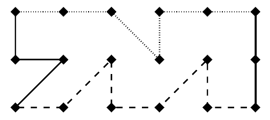
Figure 1: Dashed line: Bottom part. Pointed line: Top part.

Secondly, that means that when drawing the top or the bottom part of the polygon from left to right, only two lines of the grid may be used which means you cannot move more than one column in the opposite direction. Otherwise the way to the rightmost column could not be completed.

With these observations, we can take advantage of a left-right-ordering: We cut a valid polygon at a specified column vertically in two parts and look at the left part of it. There will be two open endings (first observation) at which we could continue to draw the polygon. Apart from the last column the shape of the left part of the polygon does not influence the number of ways we can continue to draw it, since it is not possible to go more than one column backwards (second observation).

Now we have to identify the situations or states that occur at the specified column where we made our vertical cut. With each state we associate how many possibilities we had to draw the left part of the polygon. When we find a recursive formula to get from the states of column ~i~ to the states of column ~i+1~ we can construct all possibilities from left to right, and we have basically solved the problem.

The states you choose to identify are arbitrary, as long as they are correct. A very short solution is to discard any vertical connections in the column we look at, and to associate with the upper, the middle and the lower point of the column how many connections they have to the column to the left.

State 1	State 2	State 3	State 4	State 5	State 6
~2~	~1~	~1~	~1~	~1~	~0~
~1~	~1~	~2~	~1~	~0~	~1~
~1~	~2~	~1~	~0~	~1~	~1~

One example for each state is shown in fig. 2. If we are in column ~i~ we do not need any other information than what state the left part of the polygon is in and how many possibilities we had to draw it so far. Let us denote that number with ~s_i(state)~.

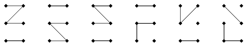
Figure 2: Examples for states ~1~, ~2~, ~3~, ~4~, ~5~ and ~6~.

Now we have to find the recurrence relationship for our ~s_i~:

$$\displaystyle \begin{align*} s_{i+1}(1) &= s_i(5) \\ s_{i+1}(2) &= s_i(5) \\ s_{i+1}(3) &= s_i(4) + s_i(6) \\ s_{i+1}(4) &= s_i(1) + s_i(2) + s_i(3) + s_i(4) + 2s_i(5) + s_i(6) \\ s_{i+1}(5) &= s_i(1) + s_i(2) + s_i(3) + s_i(4) + 2s_i(5) + s_i(6) \\ s_{i+1}(6) &= s_i(1) + s_i(2) + s_i(3) + s_i(4) + 2s_i(5) + s_i(6) \end{align*}$$

In fig. 3, all possibilities to construct state ~6~ out of the column to the left are being shown.

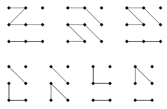
Figure 3: Recurrence relationships for state ~6~.

Let us now take a look at the possible starts, i.e. possible connections between the top and bottom part of the polygon.

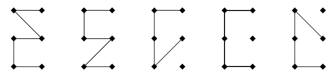
Figure 4: Possible starting configurations are states ~2~ (twice) and states ~4~, ~5~ and ~6~.

Obviously states ~1~ and ~2~ as well as states ~4~, ~5~ and ~6~ have the same recurrence relationships, and their starting values are equal, too. Therefore, it suffices to calculate states ~1~, ~3~ and ~4~:

$$\displaystyle \begin{align*} s_{i+1}(1) &= s_i(4) \\ s_{i+1}(3) &= 2s_i(4) \\ s_{i+1}(4) &= 2s_i(1) + s_i(3) + 4s_i(4) \end{align*}$$

In column ~i = N-1~ we have to close our polygon. Then the final result is ~s_{N-1}(1) + s_{N-1}(2) + s_{N-1}(5)~, i.e. ~2s_{N-1}(1) + s_{N-1}(4)~. See fig. 5 for reference.

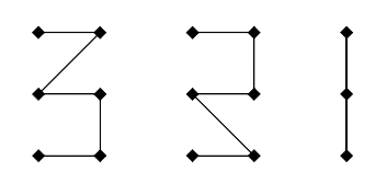
Figure 5: Possible closing configurations are states ~1~, ~2~ and ~5~.

Since the state change from column ~i~ to ~i+1~ is a linear mapping, we can do it with a matrix multiplication. In order to do that, we combine states ~1~, ~3~ and ~4~ in a vector with three components, and rewrite the recurrence relationships above as a matrix:

$$\displaystyle M = \begin{pmatrix} 0 & 0 & 1 \\ 0 & 0 & 2 \\ 2 & 1 & 4 \end{pmatrix} \quad v_{start} = \begin{pmatrix} 0 \\ 2 \\ 1 \end{pmatrix} \quad v_{end} = \begin{pmatrix} 2 & 0 & 1 \end{pmatrix}$$

Now, the problem is being solved by calculating the expression ~v_{end} M^{N-1} v_{start}~.

We could simply do ~N-1~ matrix-vector multiplications to get the result, but this is definitely too slow for ~N = 10^9~. As these multiplications are associative, we can instead calculate ~M^{N-1}~. This can be done rather quickly, namely in ~\mathcal O(\log N)~ steps:

calculateMpowerE(M, e):
  Result := IdentityMatrix;
  while (e > 0):
    if (e mod 2 == 1)
      Result = Result * M;
    M = M * M;
    e = e div 2;
  return Result;

Some math or a different state representation allows you to reduce the matrix to a ~2 \times 2~ matrix but this was not expected.

The last problem we have is that the numbers can get really big. Since only the number of possibilities modulo ~10^9~ needs to be calculated, we can do this modulo-operation on all intermediate results. They will always fit in a 64-bit integer, so there is no more trouble in that respect.

A different solution to get full score is to use a linear approach but precompute values for multiples of ~10^6~ and start the search from there.